Submitted by Norm Roulet on Sat, 06/19/2010 - 10:00.
The people of Northeast Ohio should be highly concerned about our air pollution, for many reasons. A most recent reason for concern: the May 2010 study "The Effect of Power Plants on Local Housing Values and Rents" finds "3-7 percent decreases in housing values and rents within two miles of plants with the semiparametric estimates suggesting somewhat larger decreases within one mile. In addition, there is evidence of taste-based sorting with neighborhoods near plants experiencing statistically significant decreases in mean household income, educational attainment, and the proportion of homes that is owner occupied". That is a strong analytic foundation for finding much of Cleveland is statistically worth significantly less than cleaner areas of Northeast Ohio and cities in America (as also reflected in our low property values here).

It is reasonable to project, and worth studying further, if any of the economically deflating factors in a neighborhood of NEO are found to be overlapping and cumulative, those living near multiple source points of pollution - and excessively dangerous pointsources like Mittal - should expect much larger negative impacts on property values, to the point of making private property near point sources of air pollution completely worthless... like in the neighborhoods within a few miles of Mittal.

What about the value of property within a few miles of Mittal... what does the free market think of its real value, without tax abatement, and government subsidy? We wouldn't know in Cleveland, as we have wasted all our tax and development money fighting economic reality. Read more facts about the economic realities of pollution from "The Effect of Power Plants on Local Housing Values and Rents", which is linked as a 821.04 KB .PDF file here and is copied in full below (without footnotes):
Conclusion: Electricity consumption in the United States is forecast to continue to increase over the next several decades. Although wind, solar, and other alternative sources of electricity production receive a great deal of attention from policymakers, the low cost of fossil-fuel electricity generation all but guarantees that it will play a central role in meeting this growing demand. At the same time, siting of power plants has become more difficult than ever, in large part because the need for new facilities is most severe in places with large and growing populations. Policymakers face difficult, often politically contentious decisions about where to site plants balancing many different factors. Although local amenities are typically one of the important factors considered in this process, the lack of reliable empirical evidence about the magnitude of these costs has limited the use of cost-benefit analysis.
This paper is the first large-scale effort to assess the impact of power plants on local housing markets. Across specifications the results indicate 3-7 percent decreases in housing values and rents within two miles of plants with the semiparametric estimates suggesting somewhat larger decreases within one mile. In addition, there is evidence of taste-based sorting with neighborhoods near plants experiencing statistically significant decreases in mean household income, educational attainment, and the proportion of homes that is owner occupied. Overall, however, the analysis suggests that the total local impact from power plant openings during the 1990s was relatively small because plants tended to be opened in locations where the population density is low.
That is consistent with my observations and expectations expressed on realNEO, to the outrage of this community.

If the following facts piss you off too, shut down Mittal and other polluting point sources here for real... demand real alternative energy development here... move away from pollution.... or cry to the author... he is at Haas School of Business, University of California, Berkeley, California.
The Effect of Power Plants on Local Housing Values and Rents
Lucas W. Davis - May 2010
Abstract
This paper uses restricted census microdata to examine housing values and rents for neighborhoods in the United States where power plants were opened during the 1990s. Compared to neighborhoods with similar housing and demographic characteristics, neighborhoods within two miles of plants experienced 3-7 percent decreases in housing values and rents with some evidence of larger decreases within one mile and for large capacity plants. In addition, there is evidence of taste-based sorting with neighborhoods near plants associated with modest but statistically significant decreases in mean household income, educational attainment, and the proportion of homes that is owner occupied.
Key Words: Power Plants, Hedonic Price Method, Restricted Census Microdata
JEL: D62, D63, H23, Q51
Haas School of Business, University of California, Berkeley, CA 94720-1900 and National Bureau of Economic Research.
Email: ldavis [at] haas [dot] berkeley [dot] edu.
I am grateful to Soren Anderson, Matias Busso, Dallas Burtraw, Meredith Fowlie, Michael Greenstone, Matt Kahn, Ian Lange, Matt White, two anonymous referees, and seminar participants at the University of California Energy Institute, Wharton, Resources for the Future, the Harris School of Public Policy, Michigan, Stanford, and the MIT Center for Energy and Environmental Policy Research for helpful comments.
Support from the National Institutes of Health (R03ES016608) is gratefully acknowledged. The research in this paper was conducted while the author was a Special Sworn Status researcher of the U.S. Census Bureau at the Michigan Census Research Data Center with generous guidance from Clint Carter, Jim Davis, Maggie Levenstein, Arnold Reznek and Stan Sedo. Research results and conclusions expressed are those of the author and do not necessarily reflect the views of the Census Bureau. This paper has been screened to insure that no confidential data are revealed.
1 Introduction
Electricity consumption in the United States is forecast to increase 30 percent between 2008 and 2035 according to baseline estimates from the U.S. Department of Energy. Despite growing interest in renewable energy sources, most of this growth is expected to be met with increased production from power plants using coal, natural gas, and other fossil fuels. A substantial investment in new plants has already begun with 450 new fossil fuel generators scheduled to be opened in the United States between 2010 and 2013. Nationwide over $500 billion is expected to be spent on new fossil fuel power plants between 2010 and 2030.
One of the biggest challenges in siting new plants is resistance from local communities. Citizen groups argue that power plants are a source of numerous negative local externalities including visual disamenities and noise. This paper evaluates these claims using evidence from the housing market. If households value these disamenities, then power plant openings should lead to a decrease in the price of housing in the immediate vicinity of plants. In addition, plant openings should be associated with changes in local demographics as households sort across neighborhoods based on their willingness-to-pay to avoid living near a plant. This paper tests these predictions using evidence from 92 large power plants that were opened in the United States between 1993 and 2000.
The main empirical challenge in such a study is constructing a counterfactual for the locations where power plants were opened. Power plant siting is a highly political process which, as demonstrated in the paper, leads power plants to be opened in locations near neighborhoods with particular housing and demographic characteristics. In order to better control for these differences, the analysis focuses on power plant openings rather than cross-sectional comparisons between locations with and without plants. This makes it possible to control for a rich set of demographic and housing characteristics from 1990 before the plants were opened. Some specifications also include neighborhood characteristics from 1970 and 1980 to control for differential time trends. In addition, propensity score weighting is used to equate the mean characteristics of neighborhoods in the sample with the mean characteristics of the neighborhoods near where plants were opened. This approach for mitigating omitted variables concerns is not a panacea but it offers considerable advantages over a conventional cross-sectional analysis and yields reasonable results across a range of different specifications and validity tests.
The results indicate modest declines in housing values and rents within two miles of plants. In the preferred specification, housing values decrease by 4-7 percent. Results are similar for rents, consistent with commensurate changes in current and expected future amenities. The analysis also sheds light on the evolution of neighborhood demographics near plants. Power plant openings are
associated with statistically significant decreases in mean household income, educational attainment, and the proportion of homes that is owner-occupied. These changes are consistent with taste-based sorting in which willingness-to-pay to avoid living near a plant varies across households. Again, however, the magnitude of the effects is small. For example, the analysis indicates that within two miles of plants the proportion of homes that is owner-occupied decreases by 2 to 5 percentage points compared to a mean of 68 percent.
The baseline estimates imply an average housing market capitalization of $13.2 million per plant. This is small compared to, for example, the cost of constructing new plants and reflects the fact that most plant openings during this period occurred in locations with low population density. It is important to emphasize that this capitalization captures only some of the external costs from power plants. Power plants are, for example, a major source of nitrogen oxides and other criteria pollutants that have negative impacts on human health (see, e.g., Chay and Greenstone, 2003 and Currie and Neidell, 2005). However, under normal operating conditions the vast majority of these pollutants are diluted in the atmosphere and carried far away, resulting in relatively modest disproportionate impacts in the immediate vicinity of power plants. A comprehensive analysis of the negative externalities from power plants would need to, in addition, measure these broader welfare consequences.
This study is germane to an extensive literature that examines the impact of locally undesirable facilities on housing markets. Previous studies have examined hazardous waste sites (Gayer, Hamilton and Viscusi, 2000; Greenstone and Gallagher, 2008), waste incinerators (Kiel and McClain, 1995), nuclear power plants (Nelson, 1981; Gamble and Downing, 1982), coal-burning power plants (Blomquist, 1974), and facilities that report to the Toxic Release Inventory (Bui and Mayer, 2003; Oberholzer-Gee and Mitsunari, 2006; Banzhaf and Walsh, 2008). Other studies have used similar methods to examine environmental public goods more generally including air quality (Chay and Greenstone, 2005; Bayer, Keohane and Timmins, 2009) and water quality (Leggett and Bockstael, 2000). This paper is the first large-scale study of power plants.
A key feature of this study is the use of a restricted version of the U.S. decennial census. These data, which must be accessed at a census research data center under authorization from the Census Bureau, include all of the demographic and housing characteristics in the decennial census and identify households at the census block, the smallest geographic unit tracked by the Census Bureau. This precision is important for the analysis because the impact of many of the externalities from power plants is highly-localized. In addition, the large (1 in 6) national sample ensures broad geographic coverage even in non-urban areas.
The format of the paper is as follows. Section 2 briefly reviews the hedonic price method and discusses the primary predictions of the model. Section 3 reviews relevant background about power plants focusing on externalities that are likely to be important to households living in the immediate vicinity of a plant. Sections 4 and 5 describes the data and results and Section 6 offers concluding remarks.
2 Analytical Framework
A large literature uses the hedonic price method to test whether or not households value non-
market amenities. Dozens of studies dating back at least to Ridker and Henning (1967) have used
data from the residential housing market to estimate the association between housing prices and
environmental quality. This section briefly reviews the relevant features of the hedonic model. For
a more complete description see Freeman (2003). The model provides two main testable implica-
tions. First, a decrease in environmental quality will cause housing prices and rents to decrease.
Second, households will respond to a decrease in environmental quality with taste-based sorting.
In the standard hedonic model, a differentiated good is described by a vector of characteris-
tics (z1 , z2 , ..., zn). For a house, these characteristics include structural attributes, neighborhood
amenities, local environmental quality, and other factors. Prices are determined by equilibrium
interactions between home buyers and sellers. The equilibrium relationship between prices and
characteristics is the hedonic price schedule (HPS):
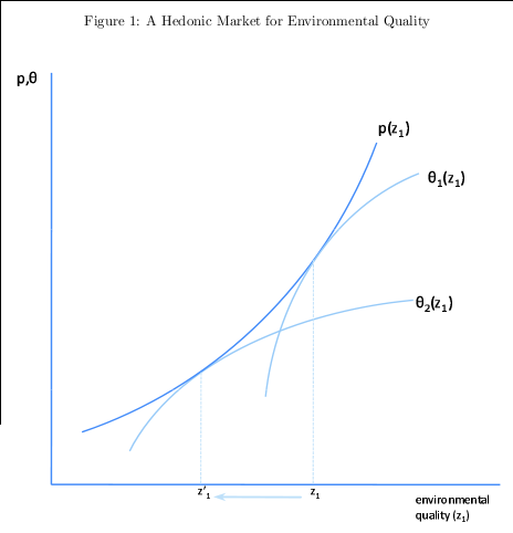
Figure 1 plots the HPS as a function of one particular characteristic, z1 , holding constant the level
of all other characteristics. Suppose z1 is a measure of local environmental quality such as distance
to the nearest power plant. If this characteristic is valued by buyers then houses in locations
with low environmental quality must have lower prices than equivalent houses in other locations
in order to attract households to these locations. The preferences of buyers are represented by
their bid function, denoted θ, an indifference curve in (p, z1) space. Utility-maximization occurs at
the point where the bid function is tangent to the HPS. The figure depicts bid functions for two
types of households. Type 1 households have strong taste for environmental quality and choose to
consume a relatively high level of z1 whereas type 2 households have weaker tastes for environmental
quality and choose a lower level. As first pointed out by Rosen (1974), at each point on the HPS the
marginal price of a characteristic is equal to the marginal willingness-to-pay (MWTP) of households
who choose to locate at that point.
For non-marginal changes in amenities the observed price differential is equal to a weighted
average of MWTP for households who choose to locate between the two points. To see this,
consider a decrease in environmental quality from z1 to z1 as indicated in Figure 1. The observed
price differential between z1 and z1 understates the MWTP of household 1 and overstates the
MWTP of household 2. The observed differential is equal to the weighted average of MWTP for
households who sort themselves into the range between z1 to z1 . It is important to note that this
is not the population average MWTP. However, from a policy perspective the population average
MWTP is often not particularly relevant. Policymakers are typically evaluating interventions that
impact a set of locations with a particular level of amenities often very different from the distribution
of amenities in the population.
In the thought experiment described above it is assumed that the HPS does not shift in response
to the decrease in environmental quality. Large-scale national changes in environmental quality will
cause the entire HPS to shift as equilibrium prices adjust to a new portfolio of housing alterna-
tives. In such cases, observed price differentials are best interpreted as the difference between two
equilibrium prices rather than a single equilibrium differential. See, e.g., Sieg, Smith, Banzhaf, and
Walsh (2005), who use a general equilibrium approach to study the effect of air quality on housing
values. For power plant openings, however, the assumption of a constant HPS is likely to be a good
approximation because only a tiny fraction of the U.S. housing market is affected. The power plant
openings between 1993 and 2000 occurred in just 92 of 65,433 total U.S. Census tracts.
A measure of the implied change in total welfare from a local decrease in environmental quality
can be calculated by multiplying the observed equilibrium price differential by the number of local
residential housing units. This measure of welfare change assumes no change in the HPS, that there
is a parallel shift in the demand curve, and that housing supply is perfectly inelastic. This last
assumption is reasonable in the short-run because housing is durable. In the long-run, a decrease
in local housing demand will also decrease the quantity of housing as older homes are razed. See
Greenstone and Gallagher (2008) for a detailed discussion of measuring welfare changes using the
hedonic price method.
In response to a decrease in environmental quality there will also be a change in the composi-
tion of local neighborhoods. Again consider a decrease in environmental quality from z1 to z1 as
indicated in Figure 1. After the decrease, type 1 households find themselves in a neighborhood
with a suboptimally low level of environmental quality and these households can increase utility
by moving to a neighborhood with the level of quality that they selected originally. After the de-
crease and subsequent sorting, households in the neighborhood will be those with relatively weaker
tastes for environmental quality. Thus, for example, if environmental quality is a normal good then
household income will tend to go down after a decrease in environmental quality. Documenting
this taste-based sorting is of significant independent interest. See, e.g. Banzhaf and Walsh (2008).
3 Background: The Local Impact of Power Plants
There are several local externalities from power plants that are likely to be important for
households living in the immediate vicinity of plants. Power plants are large industrial facilities that
can be seen from a distance because of their tall stacks. These visual disamenities are especially
acute for the large 100+ megawatt plants that are the subject of this analysis. Another local
externality from power plants is noise pollution. Fossil fuel plants produce electricity using giant
engines which generate high levels of noise and vibration. Natural gas plants use turbine engines
which can be particularly noisy. Air intake systems and cooling fans also generate noise. Although
available technologies help mitigate these problems, it is not uncommon for noise from power plants
to be heard far away, particularly during periods when plants are being tested or cleaned. Another
potential source of negative externalities from power plants is traffic from fuel deliveries. Whereas
natural gas is delivered by pipeline, coal typically arrives by train, truck, or barge. Coal plants
in the United States use over one billion tons of coal annually (over 690,000 tons per generator).5
These deliveries require thousands of trips at all hours of the day, generating noise and traffic as
well as fly ash from coal processing.
Each year power plants in the United States emit 8 million metric tons of sulfur dioxide and 3
million metric tons of nitrogen oxides, as well as other criteria pollutants.6 Under normal conditions,
however, the vast majority of these emissions are diluted in the atmosphere and carried far away.
Studies using regional atmospheric models (e.g., Levy and Spengler, 2002, Levy, et al., 2002, and
Mauzerall, et al., 2005) find little evidence of disproportionate impact on neighborhoods in the
immediate vicinity of the plant. For example, Levy and Spengler (2002) find that exposure to
health risks from sulfur dioxide and nitrogen oxides decrease approximately linearly between 0 and
500 kilometers from the source of emissions, with more than half of the social costs from emissions
borne 100 kilometers or more from the source.
Power plants also emit low levels of uranium, thorium, and other radioactive elements as well as
mercury, and other heavy metals. These toxic pollutants have been associated with serious health
problems including cognitive impairment, mental retardation, autism and blindness.8 Although
emitted in far smaller quantities than the criteria pollutants described above, these emissions have
potentially a larger impact on local communities because large airborne particles typically settle
out from the air relatively close to their emission source.9 Moreover, a small but non-negligible
amount of toxic emissions are released at ground level. Power plants in 2006 reported 1.1 million
pounds of so-called “fugitive” emissions.
Power plants also generate immense quantities of ash and other residues. When fossil fuels are
burned the noncombustible portion of the fuel is left behind along with residues from dust-collecting
systems, sulfur dioxide scrubbers and other emissions abatement equipment. These residues consist
mostly of silicon, aluminum, and iron, but also contain lead, cadmium, arsenic, selenium, mercury.
Many plants landfill these residues on site. If managed improperly, particles can be picked up by
wind and transported locally or enter drinking water supplies.
In short, power plants are the source of numerous local externalities. The baseline empirical
specification examines neighborhoods within two miles of power plants. This will tend to include the
entire area affected by visual disamenities, noise, traffic, “fugitive” emissions, and fuel residue. For
some of these local externalities, the impact would typically be even more localized. For assessing
the total welfare change, however, it is important to choose an area that is large enough so that it
includes the entire relevant area. Estimates will also be presented of the gradient of the HPS with
respect to distance. This more flexible approach provides an opportunity to empirically assess the
impact of plants at different distances.
4 Data
4.1 Power Plant Characteristics
Power plant characteristics come from the U.S. Environmental Protection Agency’s “Emissions
and Generation Resource Integrated Database (eGrid)” for 2007. This database is a comprehensive
inventory of the generation and environmental attributes of all power plants in the United States.
Much of the information in eGrid, including plant opening years, come from the U.S. Department
of Energy’s “Annual Electric Generator Report” compiled from responses to the EIA-860, a form
completed annually by all electric-generating plants. In addition, eGrid includes plant identification
information, geographic coordinates, number of generators, primary fuel, plant nameplate capacity,
plant annual net generation, and whether or not the plant is a cogeneration facility. The geographic
coordinates in the eGrid data were verified using aerial photos from Google Maps and are highly
accurate.
The sample of plants used for the main results includes all fossil fuel plants that began operation
between 1993 and 2000. This choice of years is motivated by the use of the 1990 and 2000 decennial
census data described in the following subsection. Plant construction typically takes at least two
years, making plant openings from 1991 and 1992 less valuable because information about these
plants was presumably widely available and capitalized into housing prices by 1990. In order to
evaluate the sensitivity of the results to this choice, results are also presented for plants opened
between 1993 and 1999, and plants opened between 1994 and 2000.
The analysis includes all 100+ megawatt, non-cogeneration fossil fuel plants that were opened
during this period. Plants smaller than 100 megawatts are excluded because they tend to be
built simultaneously with existing or expanding facilities such as industrial plants. Because the
objective of the study is to disentangle the disamenities from power plants it makes sense to
concentrate on these large plants that tend overwhelmingly to be independent facilities. Similarly,
cogeneration plants (i.e. plants that produce both electricity and heat, typically in the form of
steam) are excluded because they tend to be constructed simultaneously with industrial plants,
large commercial buildings, and other facilities. The sample is restricted to plants in new locations.
Existing facilities that increase the number of generators on site and plants that change their
primary energy source (e.g. switch from coal to natural gas) are excluded. Changes in capacity
and emissions levels may indeed affect the local desirability of power plants, but including these
changes in the analysis would make the results difficult to interpret. Moreover, these changes often
occur simultaneously with other changes at the plant, further complicating the interpretation of
results.
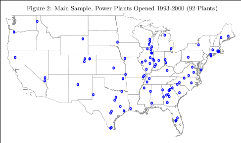
The resulting sample includes 92 plants. Figure 2 illustrates the geographic distribution. For
validity tests alternative samples were also constructed that describe all plants opened during the
1970s, 1980s, and 2003-2006.
4.2 Demographic and Housing Characteristics
Demographic and housing characteristics come from restricted census microdata for the decen-
nial census from 1990 and 2000. The primary advantage of these data is their geographic detail.
These data identify households at the Census block, the smallest geographic unit used by the Cen-
sus Bureau. An alternative to restricted census microdata would have been to use publicly-available
aggregate data for 1990 and 2000. Although basic aggregate neighborhood characteristics about
population, age and race from the short-form survey are available at the Census block level, the
more detailed information from the long-form survey including housing values, rents, and housing
characteristics for 2000 are available only at the Census block group level. Because of the focus on
highly-localized amenities it is critical to use the most disaggregated data available.
The Census Bureau’s Census 2000 Block Relationship Files were used to create geographic
identifiers linking 1990 Census blocks with 2000 Census blocks. For expositional simplicity these
linked units will be referred to as Census blocks and in cases where there is a one-to-one matching,
these units are indeed Census blocks. In cases where Census block definitions changed and the
relationship is one-to-many, many-to-one, or many-to-many, geographic identifiers correspond to
the smallest consistent geographic unit across the two surveys.
The restricted data are complemented with tract-level data from the Geolytic’s Neighborhood
Change Database for 1970 and 1980. The Geolytics data were constructed to form a panel of Census
tracts based on year 2000 Census tract boundaries. Census tracts are the smallest geographic unit
that can be matched across the 1970-2000 Censuses though in 1970 and 1980 non-urban areas
were not tracted so demographic and housing characteristics are not available for all tracts. The
Geolytics data are valuable because the 1970 and 1980 characteristics can be used to control for
time trends. These data are too coarse, however, to extend the analysis to examine plants opened
during the 1970s or 1980s. Census tracts are designed to have between 2,500 and 8,000 residents.
As a result, the land area in tracts varies widely and in non-urban areas where power plants tend
to be sited tracts can be quite large. The average land area of Census tracts with a power plant
from the sample is 193.5 square miles (median 55.7 square miles). This is the land area equivalent
to a circle with a radius of almost 8 miles.
Both the Geolytics data for 1970 and 1980 and the restricted data for 1990 and 2000 provide a
rich set of housing and demographic characteristics. The housing characteristics used in the analysis
are total owner-occupied housing units; total renter-occupied housing units; percent of total housing
units that are owner occupied; percent of total housing units that are occupied; percent of housing
units with 0, 1, 2, 3, 4, and 5 or more bedrooms; percent of total housing units that are single-unit
detached; percent of total housing units that are single-unit attached; percent of total housing units
that consist of 2, 3-4, and 5+ units, percent of total housing units that are mobile homes; percent of
total housing units built within the past year, 2 to 5 years ago, 6 to 10 years ago, 10 to 20 years ago,
20 to 30 years ago, 30 to 40 years ago, more than 40 years ago; and percent of total housing units
with all plumbing facilities. Demographic characteristics include mean household income, percent
of total persons with income below the poverty line, percent of households with public assistance
income last year, population density, percent of population Black, percent of population Hispanic,
percent of population under age 18, percent of population 65 or older, percent of population over
age 25 without a high school degree, and percent of population over age 25 with a college degree.
Housing values and rents in the census data are self-reported. With any self-reported informa-
tion one may be concerned about whether or not households are able to answer accurately. Housing
values are self-reported in response to a question that prompts respondents to report how much
they think their home would sell for if it were for sale. Particularly for owners who purchased their
homes many years ago, this may be difficult for some households to answer. In contrast, rent is
presumably not subject to the same degree of misreporting as housing values because of the saliency
of rent payments. Another potential problem with housing values is that they are reported for 20
different categories. In the empirical analysis housing value is treated as a continuous variable using
the midpoint of the range. Again, rental rates are less problematic. In 1990 rent was categorical,
but the number of categories was larger (26 categories), and in 2000 rent was a write-in response.
5 Results
5.1 Examining Covariate Balance
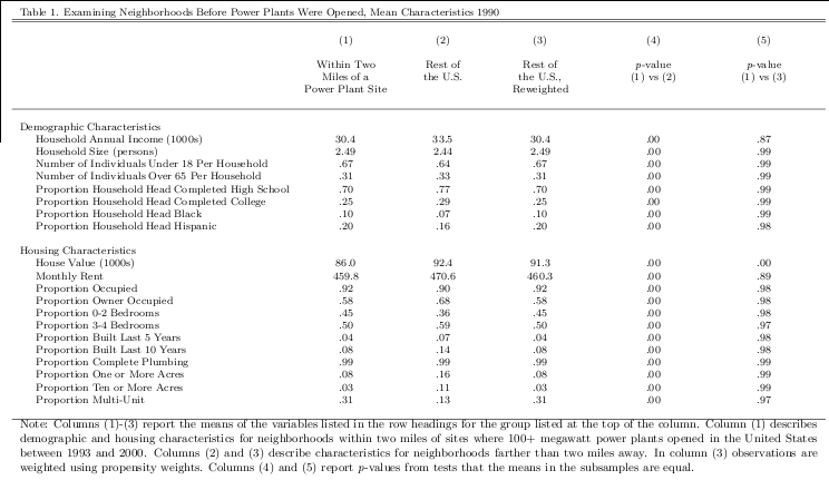
Table 1 compares neighborhoods where power plants were opened with neighborhoods in the
rest of the United States. Column (1) reports mean demographic and housing characteristics in
1990 for Census blocks for which the block centroid is within two miles of where a 100+ megawatt
power plant opened between 1993 and 2000. Column (2) describes characteristics for all other
Census blocks. Examining neighborhoods prior to when plants were opened is valuable because it
sheds light on the siting process for plants and provides evidence on the validity of the rest of the
United States as a comparison group.
Mean demographic and housing characteristics within two miles of a power plant site are sig-
nificantly different from mean characteristics for the rest of the United States. Mean household
income is lower, household size is higher, and household heads are less likely to have completed
high school or college. In addition, the proportion of households for which the household head is
black or Hispanic in the neighborhoods within two miles is higher.12 Column (4) reports p-values
from tests that the mean characteristics are equal in columns (1) and (2). The null hypothesis of
equal means is rejected in all 20 cases.
These differences underscore the importance of controlling for observable characteristics in the
analysis which follows. The main results control for these characteristics and all the other housing
and demographic characteristics listed in the previous section, as well as county fixed effects. Some
specifications also include 1970 and 1980 neighborhood characteristics to control for differential time
trends. In addition, Census blocks farther away than two miles are weighted using propensity scores.
The idea of propensity score weighting is to reweight the observations in the rest of the United
States to balance the mean characteristics of neighborhoods within two miles. Propensity scores
were estimated using a logit regression where the dependent variable is 1(within two miles), an
indicator variable equal to one for Census blocks within two miles. Regressors include all variables
in Table 1 except for housing values and rents which are often not both available for a single Census
block. Cubics were used for all variables that are not proportions (household income, household
size, number of children, and number of individuals over 65). Then, following Rosenbaum (1987),
the propensity scores from this regression were used to reweight the observations in the rest of the
United States by the relative odds

where p(Xb1990) is the conditional probability of 1−p(Xb1990 ) being within two miles given Xb1990,
the complete set of housing and demographic characteristics in 1990.
Column (3) reports means characteristics from the reweighted sample. After reweighting, means
for all covariates are virtually identical to the means in column (1) and the null hypothesis of equal
means cannot be rejected for any of the conditioning variables. Propensity weighting reduces the
potential scope for functional form misspecification in the estimating equation. Moreover, the
process of estimating a propensity score reveals the degree to which there are observations in the
rest of the United States that are similar to observations within two miles. The histograms of
the estimated propensity scores were examined and reveal a high degree of overlap between the
two groups. Although the mean propensity score is higher in the within two mile group, there are
hundreds of thousands of Census blocks in the rest of the United States with propensity scores
higher than the median propensity score in the within two mile group and tens of thousands of
Census blocks with scores higher than the 95th percentile propensity score in the within two mile
group.
5.2 Baseline Estimates of the Effect of Power Plants on Housing Values
This section presents baseline estimates of the effect of power plants on housing values and
rents. The approach is described by the following system of equations:
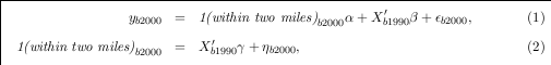
where yb2000 is the mean housing value for 2000 in Census block b (in logs). Results are also reported
for the mean rental price. The indicator variable 1(within two miles) b2000 equals one for Census
blocks in which the block centroid is within two miles of where a 100+ megawatt power plant
opened between 1993 and 2000. The coefficient of interest, α, is the price differential associated
with homes within two miles of a plant, controlling for block-level control variables, Xb1990. This
vector is restricted to variables measured in 1990 or before because variables measured in 2000
may be endogenous and reflect the impact of plant openings. In Section 5.6 several neighborhood
characteristics are examined as alternative dependent variables.
As illustrated in equation (2), power plant siting decisions or equivalently, 1(within two miles) b2000,
are postulated to be a function of location characteristics potentially including all of the character-
istics in Xb1990. Least squares estimation of equation (1) is consistent if 1(within two miles)b2000 is
exogenous conditional on Xb1990 . That is, if E[ b2000ηb2000] = 0, or that unobserved determinants
of housing prices and rents are not correlated with power plant siting decisions after controlling for
Xb1990. Estimation is consistent if, for example, power plant siting during the 1990s is a function
of housing prices, household income, educational attainment, housing characteristics, or any other
characteristic included in Xb1990. This identifying assumption is likely to be a reasonable approx-
imation given the rich set of household and demographic characteristics available in the census
data, particularly after controlling for county fixed effects. Nonetheless, it will be important in the
following subsections to evaluate the robustness of these results to alternative specifications and
validity tests.
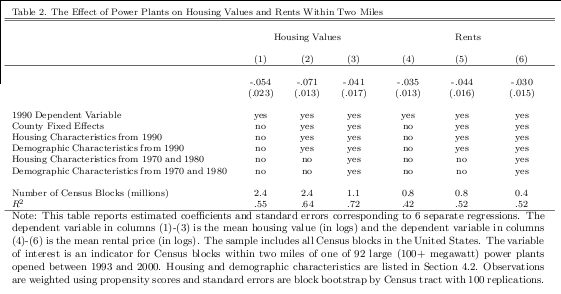
Table 2 reports least squares estimates of α for housing values and rents from three different
specifications. Columns (1) and (4) report estimated coefficients and standard errors from a spec-
ification that controls only for the 1990 dependent variable. Thus the specification in column (1)
controls for the mean housing value for 1990 (in logs) and the specification in column (4) controls for
the mean rental price for 1990 (in logs). In this specification the impact on housing values is -.054,
or -5.4 percent. The estimate for rents is also negative, with a point estimate of -.035. Columns
(2) and (5) add the complete set of housing and demographic characteristics from 1990 as well as
county fixed effects. After controlling for these additional covariates the coefficients for housing val-
ues and rents change to -.071 and -.044, respectively. Columns (3) and (6) add tract-level housing
and demographic characteristics from 1970 and 1980 to control for within-county differential time
trends. Including these lagged control variables reduces the number of observations because data
are not available for non-urban Census tracts in 1970 and 1980 and decreases the point estimates
somewhat. Overall, the point estimates indicate a decrease of 4-7 percent for housing values and
3-4 percent for rents.
Standard errors in Table 2 and throughout the paper are estimated using block bootstrap by
Census tract with 100 replications. In contrast to the point estimates which are estimated using
the complete sample of Census blocks, the bootstrap standard errors are estimated using all Census
blocks within two miles of a plant and a 5 percent random sample of all other Census blocks. For
each bootstrap sample the propensity score logit regression is reestimated in order to account for
the variance component due to estimation of the propensity scores. The confidence intervals are
fairly wide. For example, the 95 percent confidence interval for the estimate in column (1) ranges
from -.008 to -.099. Nonetheless, the estimates in all six specifications are statistically different
from zero at the 5 percent significance level. It is also possible to rule out empirically relevant
hypotheses on the high end. For example, the null hypothesis of a 10 percent decrease can be
rejected at the 5 percent significance level in all six specifications.
5.3 Total Change in Local Welfare
The estimates in Table 2 can be used to calculate a measure of the total change in local welfare
from power plant openings. In 1990 there were approximately 205,000 housing units within two
miles of locations where power plants would be opened between 1993 and 2000. The mean housing
value from Table 1 implies that the average total value of the housing stock within two miles of
a plant site is $322 million in year 2008 dollars. Multiplying this by the estimate from column
(3) in Table 2 yields an average housing market capitalization within two miles of a plant of $13.2
million. Although not negligible, this measure of the total change in local welfare is small compared
to the capital costs of a new plant. For example, to build a new coal-burning power plant costs
approximately $2000 per kilowatt of capacity so even a relatively small (100 megawatt) plant costs
$200 million. Natural gas plants are somewhat less expensive, costing approximately $1000 per
kilowatt of capacity, or $100 million for a 100 megawatt plant.13 Another point of comparison
is the cost of building electricity transmission. The typical cost of a large capacity (435 kilovolt)
transmission line is $800,000 per mile.
When interpreting this measure, it is important to keep in mind that local housing market
capitalization is a valid measure of the change in local welfare only under the assumptions outlined
in Section 2. These include that there is a parallel shift in the demand curve and that housing
supply is perfectly inelastic, for example. Also, it is important to highlight that this measure
of the change in local welfare reflects the impact on residential property but not the impact on
industrial, commercial, or undeveloped property, and thus may understate the total local welfare
change. While some industrial uses may not be substantially impacted by power plant proximity,
commercial property, and perhaps more importantly, undeveloped property, will be affected. In
addition, it is important to point out that while the results imply moderate welfare impacts on
average, there are large differences across plants in the implied market capitalization. Some of
the plants opened during this period are located in almost completely uninhabited areas whereas
others are located in relatively highly-populated areas. Finally, when interpreting this measure it
is important to remember that the local housing market capitalization reflects only some of the
externalities from fossil fuel power plants. Power plants emit sulfur dioxide and nitrogen oxides,
as well as large quantities of carbon dioxide, the principal greenhouse gas associated with climate
change. Most of the impacts of these pollutants are experienced far away from plants and are not
captured in this estimate.
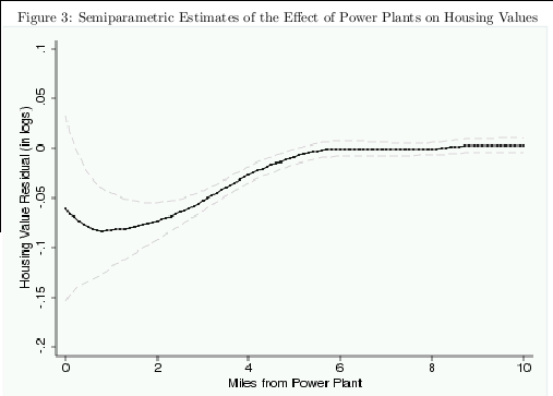
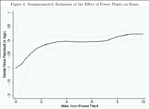
5.4 Semiparametric Estimates
Figures 3 and 4 plot semiparametric estimates of the gradient of housing values and rents with
respect to distance to the nearest power plant. First, equation (1) was estimated without the
1(within two miles) indicator. The complete set of 1990 housing and demographic characteristics
was used along with county fixed effects as in columns (2) and (5) in Table 2. Second, the gradient
with respect to distance was estimated using local linear regression with an Epanechnikov kernel
and a one-mile bandwidth.
For housing values, the point estimates start between -.10 and -.05 at the plant and then
converge to zero between one and four miles. Beyond four miles the estimates are consistently very
close to zero. For rents, the estimates start near -.10 at the plant and reach zero near two miles.
Father away from the plant the rent gradient is consistently close to zero except for a slight increase
between 8 and 10 miles. The figures also plot 95th percentile confidence intervals estimated using
block bootstrap by Census tract with 100 replications. The estimates are sufficiently imprecise,
particularly for rents to make it impossible to make definitive statements about the exact shape
of the gradient. Nonetheless, for both housing values and rents it is possible to rule out the null
hypothesis of a zero effect for at least part of the 0-2 mile range.
The lack of evidence of a housing market impact beyond a few miles is interesting because one
might have expected there to be indirect effects such as household mobility. Suppose power plants
cause households to move out of neighborhoods in the immediate vicinity of the plant but labor
market and other considerations make it undesirable for these households to move far away. These
estimates provide no evidence of such spillover effects. Still, the gradients are not precisely estimated
enough to rule out relatively small effects. The gradients are also valuable because one might have
been concerned that the impact of local externalities was obscured by employment or tax revenue
effects. According the U.S. Bureau of Labor Statistics (2008), in 2006 there were 35,000 power plant
operators in the United States. Employment from power plants increases demand for local housing,
causing a positive (and potentially offsetting) effect on housing values and rents. Similarly, power
plants are typically a substantial source of local tax revenue. The estimated gradients provide an
opportunity to evaluate these factors because whereas many of the externalities from plants are
highly localized, increased employment and property tax revenues affect all households within a
given labor or housing market. The lack of a distinguishable positive impact beyond a few miles
provides no evidence of employment or tax revenue effects, though again the estimates are not
precise enough to rule out small effects.
Overall, the semiparametric estimates are consistent with the results in Table 2 and provide
some support for the baseline empirical specification that focuses on Census blocks within two
miles of a plant. The rent gradient suggests larger effects within one mile consistent with larger
negative externalities. However, the lack of statistical precision makes it difficult to make definitive
statements about the exact shape of the gradient within two miles. Moreover, for both housing
values and rents most of the total impact appears to occur within two miles. This is particularly the
case for rents in which point estimates converge to zero almost exactly at two miles. For neither
housing values nor rents is the gradient particularly steep at two miles, suggesting that minor
changes in the specification used in Table 2 would be unlikely to substantially change the results.
5.5 Alternative Specifications and Validity Tests
Table 3 reports results for alternative specifications and validity tests. For each regression the
table reports the estimated coefficient and standard error corresponding to 1(within two miles).
All specifications are weighted using propensity scores and include county fixed effects and the
complete set of housing and demographic characteristics from 1990 as in Table 2, columns (2) and
(5).
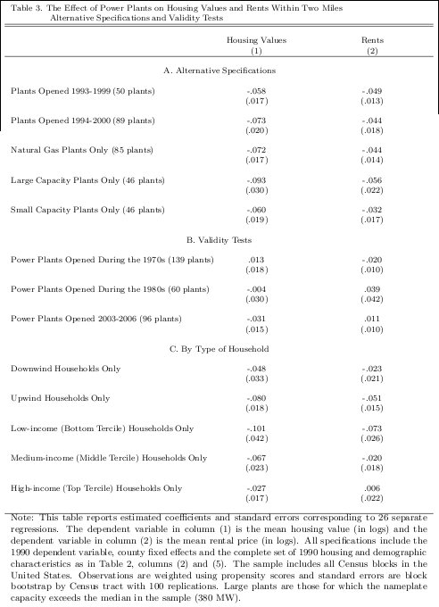
Panel A reports estimates from alternative sets of plants. First, results are reported separately
for plants that opened 1993-1999 and plants that opened 1994-2000. An unusually large number of
plants were opened in 2000 and it is reassuring that the results are not unduly sensitive to exclusion
of the plants opened in that year. Second, results are reported from restricting the sample of plants
to include only natural gas plants. Between 1993 and 2000, 85 of the 92 plant openings were
natural gas plants and restricting the sample to these plants does not meaningfully change the
estimates. It would have been interesting to report results separately for coal plants but there were
too few coal plant openings between 1993 and 2000 for the estimates to meet Census disclosure
requirements which prevent reporting coefficients based on a small number of observations. Finally,
estimates are reported separately for large and small plants. Large plants are defined as plants for
which nameplate capacity exceeds the median nameplate capacity in the sample (380 megawatts).
The point estimates indicate moderately larger effects for big plants for both housing values and
rents, though the differences are not statistically significant. It would have been valuable to more
fully characterize this relationship between plant size and local impact, or alternatively, report
estimates separately by plant. Further disaggregation would not, however, meet Census disclosure
requirements.
Panel B reports estimates from three validity tests. Instead of plants opened between 1993 and
2000, these specifications examine plants opened during the 1970s, 1980s, and 2003-2006. Because
these plants were either already open in 1990 or not yet opened in 2000 there should be no housing
market effect in 2000 after controlling for 1990 characteristics.15 As expected, the estimates are
close to zero with no consistent pattern. This lack of evidence of a relationship between these
openings and housing prices or rents is reassuring because it suggests that the results for plants
opened 1993-2000 are not driven by unobservable factors associated with the type of locations
where plants tend to be sited.
Panel C reports alternative specifications aimed at describing how estimates vary for different
types of households. First, the effect of 1(within two miles) was estimated separately for Census
blocks upwind and downwind from plants.16 The results provide no evidence of a disproportionate
impact on homes downwind of plants. If anything, there would appear to be somewhat larger
effects on upwind households but the differences are not statistically significant. Second, the effect
of 1(within two miles) was estimated separately by income tercile. The estimates are decreasing
in income, with the largest effects for Census blocks that in 1990 were in the bottom income
tercile. Again, however, these results should be interpreted with some caution because of the lack
of statistical precision.
5.6 Neighborhood Characteristics and Housing Supply
Table 4 describes the effect of power plants on neighborhood characteristics within two miles.
As described in Section 2, households will respond to a decrease in local environmental quality
with taste-based sorting. Households who place a high value on local environmental quality will
move away, while households who value local environmental quality less will move in. The table
reports estimates for 12 different dependent variables including household income, educational
attainment, demographics, housing unit characteristics, housing supply and total population using
three different specifications, all identical to the specifications used in Table 2.
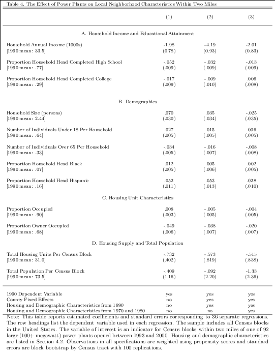
Panel A reports coefficients for household income and educational attainment. Power plant
openings are associated with between a $2000 and $4200 decrease in household annual income
within two miles of the plant. This effect is statistically significant at the two percent level in all
specifications though modest in size relative to the 1990 mean. Results for educational attainment
are similar. In columns (1) and (2) plant openings are associated with declines in the proportion
completed high school and proportion completed college. However, the point estimates change
considerably when housing and demographic characteristics from 1970 and 1980 are included. This
could indicate that the results in columns (1) and (2) are influenced by within-county differential
time trends or it could simply reflect the fact that the estimates in column (3) come from the
smaller, more urban sample for which data are available for 1970 and 1980.
Panel B reports coefficients for demographic characteristics. The estimates indicate an increase
in the number of individuals under 18 and a decrease in the number of individuals over 65 as
well increases in the proportion of household heads that are black or Hispanic. Estimates for
proportion Hispanic are positive and statistically significant at the one percent level in all three
specifications. As with educational attainment, the results in this panel are sensitive to whether or
not the specification includes characteristics from 1970 and 1980.
Panel C reports coefficients for housing unit characteristics. The estimates for the proportion
of housing units that are occupied are close to zero and not statistically significant, providing no
evidence of an increase in vacancies. For the proportion of housing units that is owner occupied,
the estimates are negative and statistically significant at the one percent level across specifications,
indicating a modest progression toward rental properties.
Finally, panel D reports coefficients for housing supply and total population. All estimates are
small relative to the mean and not statistically significant. The coefficients are estimated with
enough precision to rule out reasonably small changes in the number of housing units and total
population. The lack of evidence of a change in housing supply is perhaps not surprising because
housing is durable so a decrease in local amenities typically does not lead to an immediate decrease
in housing supply. Moreover, the direct effect of power plants on the local supply of available land
is likely to be relatively small. Even the largest power plants use at most only a few hundred acres
including all generators, the network switchyard, cooling towers and parking, typically representing
less than two percent of the total land area within a two mile radius circle around the plant.
6 Conclusion
Electricity consumption in the United States is forecast to continue to increase over the next
several decades. Although wind, solar, and other alternative sources of electricity production receive
a great deal of attention from policymakers, the low cost of fossil-fuel electricity generation all but
guarantees that it will play a central role in meeting this growing demand. At the same time,
siting of power plants has become more difficult than ever, in large part because the need for new
facilities is most severe in places with large and growing populations. Policymakers face difficult,
often politically contentious decisions about where to site plants balancing many different factors.
Although local amenities are typically one of the important factors considered in this process,
the lack of reliable empirical evidence about the magnitude of these costs has limited the use of
cost-benefit analysis.
This paper is the first large-scale effort to assess the impact of power plants on local housing
markets. Across specifications the results indicate 3-7 percent decreases in housing values and
rents within two miles of plants with the semiparametric estimates suggesting somewhat larger
decreases within one mile. In addition, there is evidence of taste-based sorting with neighborhoods
near plants experiencing statistically significant decreases in mean household income, educational
attainment, and the proportion of homes that is owner occupied. Overall, however, the analysis
suggests that the total local impact from power plant openings during the 1990s was relatively
small because plants tended to be opened in locations where the population density is low.
References
[1] Bajari, P. and C. L. Benkard, “Demand Estimation With Heterogeneous Consumers and Un-
observed Product Characteristics: A Hedonic Approach,” Journal of Political Economy 113:6
(2005), 1239-1276.
[2] Bayer, P., F. Ferreira, and R. McMillan, “A Unified Framework for Measuring Preferences for
Schools and Neighborhoods,” Journal of Political Economy 115:4 (2007), 588-638.
[3] Bayer, P., N. Keohane, and C. Timmins, “Migration and Hedonic Valuation: The Case of Air
Quality,” Journal of Environmental Economics and Management 58:1 (2009), 1-14.
[4] Banzhaf, H. S., R. P. Walsh, “ Do People Vote with their Feet?: An Empirical Test of Envi-
ronmental Gentrification,” American Economic Review 98:3 (2008), 843-863.
[5] Been, V., “Locally Undesirable Land Uses in Minority Neighborhoods,” The Yale Law Journal
103 (1994), 1383-1422.
[6] Been, V. and F. Gupta, “Coming to the Nuisance or Going to the Barrios? A Longitudinal
Analysis of Environmental Justice Claims,” Ecology Law Quarterly 24 (1997), 1-56.
[7] Blomquist, G., “The Effect of Electric Utility Power Plant Location on Area Property Value,”
Land Economics 50:1 (1974), 97-100.
[8] The Brattle Group, “Transforming America’s Power Industry: The Investment Challenge 2010-
2030,” Report Prepared for the Edison Foundation, November 2008.
[9] Bui, L. T. and C. J. Mayer, “Regulation and Capitalization of Environmental Amenities: Evi-
dence from the Toxic Release Inventory in Massachusetts,” Review of Economics and Statistics
85:3 (2003), 693-708.
[10] Busso, M. and P. Kline, “Do Local Economic Development Programs Work? Evidence from
the Federal Empowerment Zone Program,” working paper, (2008).
[11] Chay, K. Y. and M. Greenstone, “The Impact of Air Pollution on Infant Mortality: Evidence
from Geographic Variation in Pollution Shocks Induced by a Recession,” Quarterly Journal of
Economics 118:3 (2003), 1121-1167.
[12] Chay, K. Y. and M. Greenstone, “Does Air Quality Matter? Evidence from the Housing
Market,” Journal of Political Economy 113:2 (2005), 376-424.
[13] Currie, J. and M. Neidell, “Air Pollution and Infant Health: What Can We Learn from
California’s Recent Experience?” Quarterly Journal of Economics 120:3 (2005), 1003-1030.
[14] Ekeland, I., J. J. Heckman, and L. Nesheim, “Identification and Estimation of Hedonic Mod-
els,” Journal of Political Economy 112 (2004), S60-S109.
[15] Freeman, A. M. III, The Measurement of Environmental and Resource Values, Resources for
the Future, Washington D.C., 2003.
[16] Gamble, H.B. and R.H. Downing, “Effects of Nuclear Power Plants on Residential Property
Values.” Journal of Regional Science 22:4 (1982), 457-478.
[17] Gayer, T., J. T. Hamilton and W. K. Viscusi, “Private Values of Risk Tradeoffs at Superfund
Sites: Housing Market Evidence on Learning About Risk,” Review of Economics and Statistics
82:3 (2000), 439-451.
[18] Greenstone, M. and J. Gallagher, “Does Hazardous Waste Matter? Evidence from the Housing
Market and the Superfund Program,” 123:3 (2008), 951-1003.
[19] Helfand, G., “A Conceptual Model of Environmental Justice,” Social Science Quarterly 80:1
(1999), 68-83.
[20] Hirst, E. and B. Kirby, “Transmission Planning and the Need for New Capacity,” U.S. De-
partment of Energy, 2002, Washington, DC.
[21] Kahn, M. E., “Regional Growth and Exposure to Nearby Coal Fired Power Plant Emissions,”
Regional Science and Urban Economics 39 (2009), 15-22.
[22] Kiel, K. and K. McClain, “House Prices during Siting Decision Stages: The Case of an Inciner-
ator from Rumor through Operation,” Journal of Environmental Economics and Management
28 (1995), 241-255.
[23] Kohlhase, J. E., “The Impact of Toxic Waste Sites on Housing Values,” Journal of Urban
Economics 30 (1991), 1-26.
[24] Leggett, C. G. and N. E. Bockstael, “Evidence of the Effects of Water Quality on Residential
Land Prices,” Journal of Environmental Economics and Management 39:2 (2000), 121-144.
[25] Levy, J. I., J. D. Spengler, D. Hlinka, D. Sullivan, and D. Moon, “Using CALPUFF to Eval-
uate the Impacts of Power Plant Emissions in Illinois: Model Sensitivity and Implications,”
Atmospheric Environment 36 (2002), 1063-1075.
[26] Levy, J. I. and J. D. Spengler, “Modeling the Benefits of Power Plant Emission Controls in
Massachusetts,” Air and Waste Management 52 (2002), 5-18.
[27] Mauzerall, D. L., B. Sultan, N. Kim and D. F. Bradford, “NOx Emissions from Large Point
Sources: Variability in Ozone Production, Resulting Health Damages and Economic Costs,”
Atmospheric Environment 39 (2005), 2851-2866.
[28] National Oceanic and Atmospheric Administration, “National Climatic Data Center: Climatic
Wind Data for the United States,” (1998).
[29] National Research Council, “Managing Coal Combustion in Mines,” National Academies Press,
Washington D.C., 2006.
[30] Nelson, J. P., “Three Mile Island and Residential Property Values: Empirical Analysis and
Policy Implications,” Land Economics 57:3 (1981), 363-372.
[31] Oakes, J. M., D. L. Anderton and A. B. Anderson, “A Longitudinal Analysis of Environmental
Equity in Communities with Hazardous Waste Facilities,” Social Science Research 23 (1996),
125-148.
[32] Oberholzer-Gee, F. and M. Mitsunari, “Information Regulation: Do the Victims of Externali-
ties Pay Attention?” Journal of Regulatory Economics 30:2 (2006), 141-158.
[33] Rosen, S., “Hedonic Prices and Implicit Markets: Product Differentiation in Pure Competi-
tion,” Journal of Political Economy 82 (1974), 34-55.
[34] Rosenbaum, P., “Model-Based Direct Adjustment,” Journal of the American Statistical Asso-
ciation 82 (1987), 387-394.
[35] Saha, R. and P. Mohai, “Historical Context and Hazardous Waste Facility Siting: Understand-
ing Temporal Patterns in Michigan,” Social Problems 52:4 (2005), 618-648.
[36] Sieg, H., V. K. Smith, H. S. Banzhaf and R. Walsh, “Estimating the General Equilibrium
Benefits of Large Changes in Spatially Delineated Public Goods.” International Economic
Review 45:4 (2004), 1047-1077.
[37] U.S. Census Bureau, “Geographic Areas Reference Manual,” (1994).
[38] U.S. Bureau of Labor Statistics, U.S. Department of Labor, “Occupational Outlook Handbook,
2008-09 Edition, Power Plant Operators, Distributors, and Dispatchers,” (2008).
[39] U.S. Department of Energy, Energy Information Administration, “Assumptions to the Annual
Energy Outlook 2009,” (2009), DOE/EIA-0554.
[40] U.S. Department of Energy, Energy Information Administration,“Annual Energy Outlook
2010: With Projections to 2035,” (2010a), DOE/EIA-0383.
[41] U.S. Department of Energy, Energy Information Administration, “Electric Power Annual
2008,” (2010b), DOE/EIA-0348.
[42] U.S. Department of Health and Human Services, “ToxFAQs,” (2007).
[43] U.S. Environmental Protection Agency, “The Particle Pollution Report: Current Understand-
ing of Air Quality and Emissions through 2003,” (2004), EPA 454-R-04-002.
[44] U.S. Environmental Protection Agency, “Mercury Study Report to Congress, Volume III: Fate
and Transport of Mercury in the Environment,” (1997), EPA 452-R-97-005.

